Index page

Differentiable Programming

Deep Learning is dead. Hello Differentiable Programming. (Uh come on man)

In theory

So what was deep learning and why did we move on? Or did we? In summary, DL had the following steps -> Pick a bunch of inputs and outputs -> Start off by randomly defining a relationship -> Pass it through neural network -> perform gradient descent -> Optimize a loss function -> Repeat until it either works or blows up.

Now what? Well now we take this and realize that hey! What if we applied this to code itself??!! Crazy right? All it means is, why not take arbitrary (almost) code and if it can be differentiated, calculate its gradient and.. optimize it for a function!

Does that make sense? I guess not. So in other words. We can take existing equations which we say know parts of and then use this approach to fill in so to speak. What does this mean? We can apply domain knowledge and well defined laws and use data to find equations to model our system!

Say we have simulated a physics engine (many exist) and we run a simulation. Using a Neural ODE we can plug in the variables we need and compute an equation. "Theoretically"

I am still figuring things out so I will update this as I go along. If I get anything wrong now, hopefully I will learn enough to fix it. If not, please do tell me

Lotka Volterra

As an example, here is the most common one I found so far. The Lotka Volterra model. What is it? Simply put, it is an ecological model which tries to describe the relationship between two species where one is a predator and the other is prey. It aims to model how the population changes over time.

Here we get some different packages. Along with our old friends Latexify, Flux and Plots. DiffEqFlux will allow us to use differential equation solvers. I do not think I will try to implement that from scratch as it is currently wayy out of scope for me. The only major thing I will try to atleast understand and write in depth about is Automatic Differentiation. (More explained throughout the course of this article)

using Latexify
using DiffEqFlux, DiffEqSensitivity, Flux, OrdinaryDiffEq, Zygote, Test
using Plots

What is it

Okay now let us model the system.

We have two populations and so we need two starting values which we set as x and y. We will also define a few parameters that we need. The first being the equation of the first population.

We take α to be the growth rate.
β to be the rate at which the prey is killed.
δ to be the death rate of the predators
γ rate at which the predators increase

$$dx = \left( \alpha - \beta \cdot y \right) \cdot x$$

The second being the equation of the second population.

$$dy = \left( \delta \cdot x - \gamma \right) \cdot y$$

function lotka_volterra(du,u,p,t)
    x, y = u
    α, β, δ, γ = p
    du[1] = dx = (α - β*y)x
    du[2] = dy = (δ*x - γ)y
end

Modelling it

Now that we have a model of our system, we set a few default values just to start with. Giving the inital populations a value of 1. And some default parameters for our rates.

We then pop this into what is known as an ODEProblem. This is a wrapper for allowing us to pose our function as an ODE. We can then attempt to solve it using an ODESolver. (I am still getting the details. When I understand it fully, there will be a post)

p = [2.2, 1.0, 2.0, 0.4]
u0 = [1.0,1.0]
prob = ODEProblem(lotka_volterra,u0,(0.0,10.0),p)

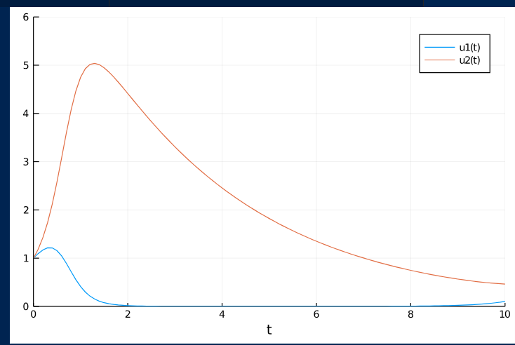
Our current plot looks something like this. -

So we write a tiny function to return an array with the solutions for that current timestep. We are also using the Tsit5(Tsitorous) solver. This seems to be part of something called Runge-Kutta. A google says "Runge–Kutta method is an effective and widely used method for solving the initial-value problems of differential equations and can be used to construct high order accurate numerical method by functions' self without needing the high order derivatives of functions.".

I guess that roughly translates to -> Solve a higher order differential equation without much overhead?

function predict_rd()
    Array(solve(prob,Tsit5(),saveat=0.1,reltol=1e-4))
end

Now for something more up my alley. Optimizers and loss!! We are using sum of squared absolute error here it seems. And our dear friend Adam. We also have a callback function to display the current loss and then try to remake the equation using the current parameters so we can plot it.

loss_rd() = sum(abs2,x-1 for x in predict_rd())

opt = ADAM(0.1)

cb = function ()
  display(loss_rd())
  display(plot(solve(remake(prob,p=p),Tsit5(),saveat=0.1),ylim=(0,6)))
end

Train!!

Finally we can train the network.

Flux.train!(loss_rd, Flux.params(p), Iterators.repeated((), 100), opt, cb = cb)

Outputs

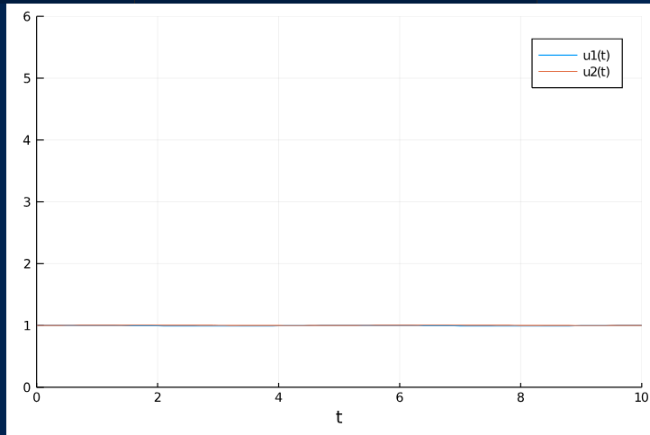
As time goes by we get. - -

And finally.

Yay! We have successfully modelled an equation using a neural network with barely any data. This is a first step duh. Long way to go before I get anywhere substantial. But baby steps right?

Home page